Example I. Logistic Regression:
Adherence in a Pharmacy Assistance Program
Methods:
We used a retrospective cohort design to investigate six-month outcomes for participants in the University of North Carolina (UNC) Health Care Pharmacy Assistance Program (PAP) who received medications indicated for hypertension, diabetes, and/or hyperlipidemia from 2009 through 2011. The three study cohorts included 866 patients receiving antihypertensive agents, 265 patients receiving oral glucose-lowering agents, and 455 patients receiving statins. Multivariable logistic regression was used to examine the impact of the predefined covariates on medication adherence (primary outcome).
Adjusted Multivariable Logistic Regression Results Predicting Adherencea Among Newly Enrolled Participants in the UNC Health Care Pharmacy Assistance Program to Medications for a Specific Chronic Disease
| Characteristic / Variable Predicting Adherencea |
Users of Antihypertensive Agents (N = 866) OR (95% CI) |
Users of Oral Glucose-Lowering Agents (N = 265) OR (95% CI) |
Users of Statins (N = 455) OR (95% CI) |
| Age |
1.03** (1.01 – 1.04) |
1.02 (0.99 – 1.05) |
1.04* (1.00 – 1.05) |
| Female sex |
0.84 (0.63 – 1.13) |
0.70 (0.42 – 1.18) |
0.74 (0.49 – 1.10) |
| White race |
0.89 (0.65 – 1.22) |
1.83* (1.05 – 3.21) |
1.82** (1.19 – 2.79) |
| English as preferred language |
0.74 (0.48 – 1.12) |
1.07 (0.53 – 2.14) |
1.21 (0.64 – 2.32) |
| Local residenceb |
1.31 (0.96 – 1.79) |
1.37 (0.76 – 2.47) |
1.23 (0.79 – 1.92) |
| No. of unique drugs received |
1.17** (1.13 – 1.22 |
1.05 (0.99 – 1.11) |
1.06** (1.02 – 1.11) |
| Use of any hypertensive agent |
– |
1.17 (0.64 – 2.13) |
1.36 (0.85 – 2.16) |
| Use of any glucose-lowering agent |
1.20 (0.81 – 1.79) |
– |
1.37 (0.89 – 2.12) |
| Use of any statin |
1.80** (1.30 – 2.49) |
1.75 (0.99 – 3.10) |
– |
CI = confidence interval
OR = odds ratio
UNC = University of North Carolina
*P < .05
**P < .01
aAdherence was defined as having an overall, aggregate proportion of days covered (PDC) equal to or greater than 0.8 for medications within a cohort.
bLocal residence was defined as living in one of these seven counties: Orange, Chatham, Alamance, Caswell, Person, Durham, or Wake.
Results:
When all covariates were included, older age was a statistically significant predictor of adherence to antihypertensive agents (OR = 1.03; 95% CI, 1.01 – 1.04) and adherence to statins (OR = 1.03; 95% CI, 1.00 – 1.05). Similarly, the number of unique medications for which prescriptions were filled also had a statistically significant positive association with adherence to antihypertensive agents and with adherence to statins. White race was associated with 83% greater odds of adherence to oral glucose-lowering agents (OR = 1.83; 95% CI, 1.05 – 3.21) and 82% greater odds of adherence to statins (OR = 1.82; 95% CI, 1.19 – 2.79). For patients in the antihypertensive cohort, concomitant use of statins significantly increased the odds of adherence to antihypertensive agents. Patient sex, language preference, and local residence were not associated with adherence to medications for any of the 3 cohorts.
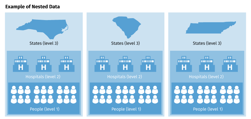
Example II. Multilevel Model:
Variance in individual health status attributable to the family
Methods:
Secondary data were used from the Community Tracking Study. Participants were US residents aged 18 years and older who shared a household with family members in the study (N = 35,055). Main outcome measures were the Short Form-12 (SF-12) self-reported physical subscales. Hierarchical linear modeling was used to estimate the individual and family components of health status. The setting was 60 US communities, which account for approximately one half of the population. Our initial analysis used the combined level-3 model to partition the variance of the SF-12 scores into 3 components: individual (level-1), family (level-2), and community (level-3). Because the community level accounted for less than 1% of the total variance in health status scores in initial analyses, however, subsequent analyses were limited to the individual (i.e., level-1) and family (i.e., level-2) components. The second analysis was a series of multilevel regression equations that sequentially added age, family income, and then health insurance status as predictors of SF-12 scores. For this set of equations, we were interested in assessing the proportion of family-level variance accounted for as each covariate was added to the model.
Table 2: Multilevel Variance Components for SF-12 Physical Health Summary Score
|
Individual |
Family |
| Family Composition |
Level-1 Var |
SE |
% |
Level-2 Var |
SE |
% |
| Single-family households |
|
|
|
|
|
|
| Married, no kids |
88.48 |
4.43 |
77.7 |
25.43 |
3.72 |
22.3 |
| Married with kids |
55.14 |
3.11 |
86.8 |
8.44 |
2.00 |
13.2 |
| Single with kids |
77.59 |
11.13 |
76.9 |
23.31 |
9.38 |
23.1 |
| Multiple-family households |
|
|
|
|
|
|
| Married, no kids |
103.05 |
11.50 |
83.9 |
19.85 |
8.65 |
16.1 |
| Married with kids |
70.66 |
9.20 |
83.9 |
13.53 |
6.33 |
16.1 |
| Single with kids |
75.93 |
14.64 |
95.5 |
3.64 |
9.16 |
4.5* |
Var = variance
SE = standard error
SF-12 = short form 12
*Not significant
Table 4: Multilevel Regression Parameters (Regression Weight and SE) for SF-12 Physical Component Summary Scores in Single Family Households
| Family Composition |
Intercept |
Age Years |
Income* |
Insurance Status† |
Level-2 Variance, % |
–2*logL‡ |
| Married, no kids |
|
|
|
|
|
|
| Model 1 |
48.05 (0.23) |
– |
– |
– |
22.3 |
89,725 |
| Model 2 |
58.11 (0.63) |
–0.18 (0.02) |
– |
– |
16.2 |
88,942 |
| Model 3 |
50.93 (1.10) |
–0.15 (0.02) |
1.65 (0.15) |
– |
12.5 |
88,510 |
| Model 4 |
48.75 (1.30) |
–0.13 (0.02) |
1.47 (0.20) |
1.25 (0.42) |
12.6 |
88,452 |
| Married with kids |
|
|
|
|
|
|
| Model 1 |
51.82 (0.16) |
– |
– |
– |
13.2 |
105,957 |
| Model 2 |
54.62 (0.62) |
–0.08 (0.02) |
– |
– |
13.5 |
105,851 |
| Model 3 |
51.06 (0.74) |
–0.10 (0.02) |
1.28 (0.16) |
– |
10.1 |
105,398 |
| Model 4 |
50.65 (0.80) |
–0.10 (0.02) |
1.19 (0.16) |
0.44 (0.14) |
9.9 |
105,376 |
| Single with kids |
|
|
|
|
|
|
| Model 1 |
49.62 (0.54) |
– |
– |
– |
23.31 |
16,289 |
| Model 2 |
53.91 (1.72) |
–0.13 (0.06) |
– |
– |
22.05 |
16,257 |
| Model 3 |
50.80 (1.73) |
–0.17 (0.06) |
2.14 (0.42) |
– |
8.8§ |
16,141 |
| Model 4 |
50.51 (1.88) |
–0.017 (0.06) |
2.03 (0.46) |
0.39 (1.62)§ |
8.6§ |
16,137 |
SF-12 = short form 12
*Income quintile: 1 = lowest; 5 = highest
†Insured
‡-2*LogL is a goodness-of-fit statistic. Smaller numbers indicate a better model fit.
§Not significant
Results:
The family (i.e., level-2) variance component ranged from 4.5% to 26.1% for the physical health score. All the level-2 variance components for physical health were statistically significant except for single persons with children in multiple-family households. As seen in Table 4, age and income were significant predictors of physical health status in all family configurations. The effects were in the expected direction; older age, lower income, and lack of insurance were associated with worse physical health status. Age accounted for approximately 30% of the level-2 variance for physical health status in the “married, no kids” group, reducing the family-level variance component from 22.3% to 16.2% of the total variance. This magnitude of effect was not observed in the “married with kids” or the “single with kids” groups. Adding income to the regression equations further reduced the level-2 variance component by 23% to 60% in all family configurations. After adjustment for age and income, insurance status only slightly improved the model.
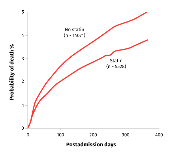
Example III. Survival Analysis:
Statin Treatment and 1-year Survival
Methods:
Prospective cohort study using data from the Swedish Register of Cardiac Intensive Care on patients admitted to the coronary care units of 58 Swedish hospitals in 1995 – 1998. Participants included patients with first registry-recorded AMI who were younger than 80 years and who were discharged alive from the hospital, including 5,528 who received statins at or before discharge and 14,071 who did not.
Main Outcome Measure Relative risk of 1-year mortality according to statin treatment.
Comparisons between different patient strata and different categories of hospitals were analyzed by χ2 tests for categorical variables and by the t-test for continuous variables. Bivariate analyses and multiple covariate Cox regression analyses were used to identify any variable with a significant influence on mortality. The analyses were also performed for 30-, 60-, and 90-day survivors to allow for even longer periods of early mortality in patients who could have been perceived to have a too-short life expectancy to benefit from statin treatment.
Figure. Adjusted Probability of Mortality by Statin Treatment:
Click here for a detailed description.
Results:
Among the 14,071 patients without statin treatment, the unadjusted 1-year mortality was 9.3% (n = 1,307) compared with 4.0% (n = 219) among the 5,528 patients with statin treatment. In Cox regression analysis, adjusting for the 43 covariates, statin treatment at discharge was associated with a reduction in 1-year mortality (3.7% vs 5.0%; relative risk [RR], 0.75; 95% confidence interval [CI], 0.63 – 0.89; p = .001)