Lesson 5: Continuous Outcomes, Between Groups Differences

This lesson reviews between-group differences for a data set containing a continuous or ordinal dependent and discrete independent variables. At the end of this lesson, you will be able to:

Describe the one-sample t-test, two-sample t-test, paired t-test, and one-way ANOVA
Describe the non-parametric equivalents of each test above
Describe the Bonferonni correction
Interpret the results of a test comparing group means

Terms that appear frequently throughout this lesson are defined below:

Term	Definition
One Sample t-test	A test that compares the mean score of a sample to a known value, typically the population mean
Student t-test	A test to determine the probability that the difference in two group means happened by chance. Also called the independent samples t-test or two sample t-test
Mann-Whitney U	The non-parametric equivalent of the student t-test
Paired t-test	A test that examines the difference between paired values in two samples (e.g., a pre and post-test)
Wilcoxon Matched-Pair test	The non-parametric equivalent of the paired t-test
Analysis of variance (ANOVA)	A test to determine the probability that the difference in three or more group means happened by chance
Kruskal-Wallis One-Way ANOVA	The non-parametric equivalent of the ANOVA
Bonferonni correction	An approach to reducing the statistical significance level when multiple comparisons are made on the same set of data

Three samples of one population

I. One sample t-test

The one-sample t-test compares the sample mean of a single group to the population mean to determine if the probability that the sample is different from the population could have occurred by chance. For example:

Comparing the mean PCAT score for a cohort of students to the national PCAT average
Comparing the mean birthweight of babies born to poor women in a prenatal care program to the expected birthweight of babies born to poor women

II. Student t-test

Also called independent samples t-test, two-sample t-test, and unpaired t-test.

The student t-test compares the means of two independent samples to determine if the probability that the difference between the two means could have occurred by chance. For example:

Comparing the mean outcome of a group randomly assigned to a treatment to the mean outcome of another group from the same sample assigned to a non-treatment group
Comparing the mean outcome for male participants to the mean outcome for female participants

The primary assumptions when running a student t-test include:

Samples are independent. In other words, if an individual’s data is used to calculate one sample mean, it should not be included in the other sample mean.
Population data from which the sample is drawn is normally distributed.
Variances are approximately equal.

Mann-Whitney U

The non-parametric equivalent to the student t-test looks at the relative rank of the subjects in the two groups. It is generally used if data is highly skewed (i.e., non-normal), ordinal, and/or for small sample sizes (e.g., convention: n < 30). Exact tests should be used if any expected frequencies are less than five.

III. Paired t-test

Also called paired difference t-test

The paired t-test compares the means of two dependent samples to determine if the probability that the difference between the two means could have occurred by chance. For example:

Comparing the mean outcome of a group at time 1 (pre) and at time 2 (post)
Comparing the mean outcome for blood pressure measurements using a stethoscope and blood pressure measurements using a dynamap with the same participants in receiving both measurements

Wilcoxon Matched-Pairs Test

Also called Wilcoxon signed-rank test

The non-parametric equivalent to the paired t-test looks at the differences in ranks between the two measures. It is generally used if data is ordinal, and/or for small sample sizes (e.g., convention: n < 30). Exact tests should be used if any expected frequencies are less than five.

IV. One-way ANOVA

The one-way analysis of variance (ANOVA) compares the means of three or more independent samples to determine if the probability that the difference between means could have occurred by chance. For example:

Comparing the mean outcome of a group using Drug 1, a group using Drug 2, and a group using Drug 3
Comparing the mean outcome of a group with Disease 1, a group with Disease 2, a group with Disease 3, and a group with Disease 4

Post-hoc tests

When a significant difference is found by an ANOVA, it is helpful to know which groups in the test differed significantly from one another. Groups 1 and 2 may differ significantly, but groups 1 and 3 may not. A post hoc analysis can identify which means are significantly different from each other. Common tests include Least Significant Difference (LSD), Tukey’s HSD, and Bonferroni. The Bonferonni uses the Bonferroni correction, is generally considered the most conservative, and is widely favored in the health sciences.

Bonferroni correction adjusts for multiple comparisons made with the data. Making multiple comparisons (e.g., comparing the means of many different groups) increases the likelihood of finding a significant difference, increasing the chances that we will reject the null hypothesis even when its true. The Bonferroni correction simply divides alpha by the number of comparisons being made. If eight comparisons are being made for an outcome, then the Bonferroni correction would make alpha = 0.05/8 = 0.00625.

Kruskal Wallis

The non-parametric equivalent to ANOVA looks at the differences in ranks between more than two groups. It is generally used if data is highly skewed (non-normal), ordinal, and/or for small sample sizes (e.g., convention: n < 30). Exact tests should be used if any expected frequencies are less than five.

Repeated measures ANOVA

The repeated measures ANOVA compares the means of three or more dependent samples to determine if the probability that the difference between means could have occurred by chance. Examples include: comparing the mean outcome of a group at four separate points in time.

Example 1: Medication Adherence in Managed Care

Consider the following table. Which statistical tests could be used to examine differences between groups?

Patient Cohort Demographic Characteristics and Drug Utilization Metrics by Index Drug Class*

Characteristic	Metformin (n = 1274)	Sulfonylureas (n = 1081)	Thiazolidinediones (n = 337)	Total^† (n = 2741)
Age, y	53 ± 11	55 ± 12	52 ± 11	54 ± 11
Female, %	54	49	51	49
CDS	2.89 ± 0.96	2.85 ± 1.0	2.99 ± 0.97	2.89 ± 0.99
Patients with > 1 fill of index drug, n (%)	1001 (78.6)	861 (79.6)	264 (78.3)	2126 (77.6)
Adherence, %^‡	80.7 ± 21.6	81.8 ± 21.7	82.0 ± 21.4	81.3 ± 21.6
Adherence ≥ 80%	63.9%	65.8%	69.4%	65.4%

*Data are given as mean ± SD unless otherwise indicated.
†Because of small sample size, results for patients whose index drug was an α-glucosidase inhibitor or a meglitinide (n = 49) are not presented by index drug category in the table, although they are included in the “Total” column.
‡Adherence was calculated for the patient subset with at least two fills of the index drug(s).
CDS indicates chronic disease score.

Nominal (categorical) variables:

Drug class (i.e., Metformin, Sulfonylureas, Thiazolidinediones)
Gender (i.e., Female, not female)
Patients with > 1 fill of index drug (i.e., Yes, No)
Adherence >=80% (i.e., Yes, No)

Continuous variables:

Age
CDS
Adherence

Test selection includes:

Chi-square (this test will be covered later in the module)

Gender by drug class
Patients with >1 fill of index drug by drug class
Adherence >=80% by drug class
Adherence >=80% by gender

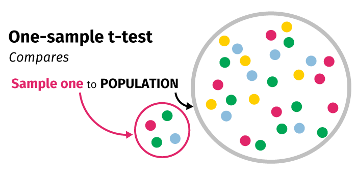
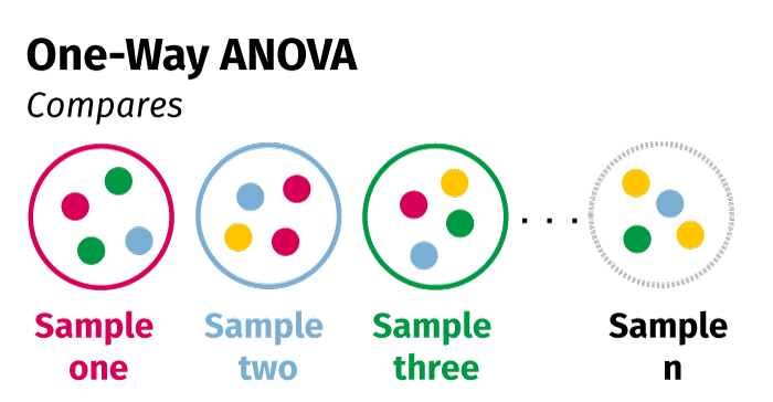
T-test (two groups) or One-Way ANOVA (three or more groups)

Age by drug class
CDS by drug class
CDS by adherence >=80%
Adherence by drug class

Methods:

Continuous data were described by means and standard deviations, and categorical data were described by frequencies and percentages. Demographic, clinical, and medication characteristic comparisons between groups were completed by using t-tests, analysis of variance, and correlation analysis for evaluation of continuous variables and the χ² test for categorical variables.

Example of Results:

The mean CDS overall was 2.89 ± 0.99, with a small but significant difference between SU and TZD patients (2.85 vs 2.99, p = .04). Mean adherence for the study cohort was 81% and did not significantly differ by therapeutic class. Older patients were more likely to be adherent (i.e., mean age 56 years vs 52 years, p < .0001), but there was no difference between men and women in adherence (p = .61). Adherent patients had a significantly higher disease burden, as measured by CDS (2.99 vs 2.86, p = .0022).

Rozenfeld Y, Hunt JS, Plauschinat C, Wong KS. Oral antibiotic medication adherence and glycemic control in managed care. Am J Manag Care. 2008; 14: 71-75.

Example 2: Medication Adherence in Medicare Part D Programs

Consider the following table. Which statistical tests were used to calculate these p-values?

Relationship Between Potential Predictors and Nonadherence* to Three Classes of Medications Among
Medicare Part D Enrollees with Diabetes from Six States.
(Data are percentages^†, except as indicated.)

Patient Characteristic	Adherent	Not Adherent	P	Adherent	Not Adherent	P	Adherent	Not Adherent	P
	Oral Hypoglycemic Agents			ACEIs/ARBs			Statins
Age, y
< 65	14.7	19.7	< 0.001	14.1	18.4	< 0.001	14.4	18.8	< 0.001
65 – 74	44.5	41.8	< 0.001	43.6	41.2	< 0.001	44.7	43.1	< 0.001
≥ 75	40.9	38.5	< 0.001	42.3	40.5	< 0.001	40.9	38.1	< 0.001
Sex
Male	42.3	40.5	< 0.001	40.5	38.6	< 0.001	42.1	39.8	< 0.001
Female	57.9	59.5	< 0.001	59.6	61.4	< 0.001	57.9	60.2	< 0.001
Race/ethnicity
White	67.7	62.0	< 0.001	67.1	60.5	< 0.001	69.0	65.2	< 0.001
Black	14.5	19.4	< 0.001	15.5	20.4	< 0.001	12.9	15.9	< 0.001
Hispanic	7.5	9.4	< 0.001	7.3	9.5	< 0.001	6.9	9.1	< 0.001
Other	10.3	9.2	< 0.001	10.2	9.6	< 0.001	11.4	9.8	< 0.001
Deyo-adapted CCI, mean (SD)	0.9 (1.7)	1.3 (2.1)	< 0.001	1.1 (1.9)	1.6 (2.3)	< 0.001	1.1 (1.9)	1.5 (2.2)	< 0.001

ACEIs = angiotensin-converting enzyme inhibitors; ARBs = angiotensin II receptor blockers; CCI = Charlson Comorbidity Index
*Nonadherence was defined as proportion of days covered < 80%.
^†Columns may not add to 100% because of rounding.

Nominal (categorical) variables:

Drug class (Oral hypoglycemic agents, ACEIs/ARBs, statins)
Age (<65, 65 – 74, >=75)
Sex (male, female)
Race/Ethnicity (White, Black, Hispanic, Other)
Adherence (adherent, not adherent)

Continuous variables:

Deyo-adapted CCI

Test Selection includes:

Chi-square

Age by adherence to oral hypoglycemic agents
Age by adherence to ACEIs/ARBs
Sex by adherence to oral hypoglycemic agents
Sex by adherence to ACEIs/ARBs
Race/ethnicity by adherence to oral hypoglycemic agents
Race/ethnicity by adherence to statins

T-test (two groups)

Deyo-adapted CCI by adherence to oral hypoglycemic agents
Deyo-adapted CCI by adherence to ACEIs/ARBs
Deyo-adapted CCI by adherence to statins

Methods:

The relationship between medication nonadherence and patient characteristics was evaluated using χ² tests for categoric variables and t-tests for continuous variables.

Example of Results:

Patients aged <65 years, women, black or Hispanic patients, and patients with higher comorbidity scores (Deyo-adapted CCI) were more likely to be nonadherent to oral hypoglycemic agents, ACEIs/ARBs, and statin medications (Table II).

Yang Y, et al. Predictors of medication nonadherence among patients with diabetes in Medicare Part D programs: a retrospective cohort study. Clinical Therapeutics. 2009; 31(10): 2178-2188.