| Term |
Definition |
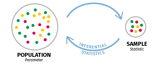
| Population |
The entire collection of people, animals, cells, or other things from which we collect data |
|
Parameter
|
A number that is calculated from an entire population |
| Sample |
A subset or group drawn from the population |
|
Statistic
|
A number or quantity that is calculated from a sample of data |
|
Descriptive statistics
|
Statistics that describe the sample without attempting to generalize the results to other groups or the population |
|
Inferential statistics
|
Statistics that infer the likelihood that the results can be generalized to the population |
| Measure of central tendency |
A single value that attempts to describe the central position of a set of data |
|
Mean
|
The average value |
|
Median
|
The middle value |
|
Mode
|
The most frequent value |
| Measure of dispersion/variation |
A value that describes how the data are dispersed around the measure of central tendency, or the extent to which individual values differ from the mean, median, or mode |
|
Standard deviation
|
On average, how much individual values differ from the mean; the square root of the variance |
|
Variance
|
How far a set of numbers is spread out from the mean; the sum of the squared differences between each value and the mean, divided by the number of values minus one |
|
Range
|
The difference between the largest and smallest value in the data set |
|
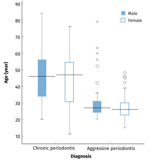
Interquartile range
|
A measure of the “middle fifty” in the data set; where the bulk of the values exist |
|
Outlier
|
An observation point that is distant from other observations |
|
Frequency
|
The number of times a value appears in the data set |
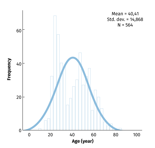
| Frequency distribution |
A table or graph that illustrates how frequently each value appears in the data set |
|
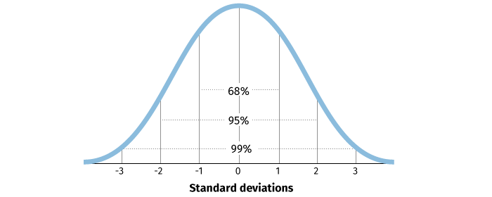
Normal distribution
|
A symmetric, bell-shaped distribution for a continuous variable; 68% of observations fall within 1 standard deviation of the mean, 95% fall within 2 standard deviations of the mean, and 99.7% fall within 3 standard deviations of the mean |
|
Binomial distribution
|
The probability distribution for a binomial variable (i.e. a variable that has only two possible values) with fixed probabilities that add up to one |
|
Confidence interval
|
An estimate of the population parameter that will contain the population mean a specified proportion of the time, typically either 95% or 99% of the time |
|
Probability
|
The likelihood that an event will occur |